
Solution, reactions and equilibrium
Linear statics finds nodal displacements for which internal elastic forces balance the external load. Zero prescribed displacements allow solving only the free part without changing the full stiffness matrix.
Full and reduced systems
Original equation:
K u = F + R
Here R denotes support reactions. Partition rows and columns into free f and constrained c:
In FEM, a free degree of freedom is a nodal translation or rotation whose value is not prescribed by boundary conditions and must be determined by analysis. The term refers to an individual displacement component, not to the entire node. It does not imply motion without resistance: elements connected to the node may deform and develop elastic forces. For example, the unsupported end of a cantilever frame has free X and Y translations and a free rotation, but the cantilever stiffness resists these motions.
[ Kff  Kfc ] [ uf ] = [ Ff ] + [  0 ]
[ Kcf  Kcc ] [ uc ]   [ Fc ]   [ Rc ]
For the implemented homogeneous supports, uc = 0. The first block row becomes a system for the unknown free displacements:
Kff uf = Ff
Loads applied to constrained DOFs do not enter the reduced right-hand side but remain in the full F and are included in reaction recovery.
Checks before solving
validateReducedSystem checks coefficient finiteness and positive definiteness of the symmetrized Kff using Cholesky factorization. Failure usually means one of two things:
- insufficient supports allow rigid-body motion;
- an internal mechanism remains, for example a node can move transversely to every connected truss member without extending them in the linear approximation.
For a unique solution to the linear static problem considered here, the supports and element stiffness must exclude rigid-body motions and internal mechanisms — possible motions without elastic resistance. Free DOFs are allowed: the corresponding unknown displacements are determined from the equilibrium equations Kffuf = Ff, and reactions are calculated after solving. A fully constrained model is a valid special case: with zero prescribed displacements, there are no free DOFs, all displacements are zero, and reactions balance the applied loads.
Expanding to the full vector
After solving the reduced system, a zero vector of length n is created and the computed components are inserted at indices freeDOFs:
u = zeros(numberOfDOFs, 1);
u(freeDOFs) = K(freeDOFs, freeDOFs) \ F(freeDOFs);
The full vector is needed to recover element strains, reactions and results at any node. Constrained components remain exactly zero.
Reactions and global equilibrium
After expanding the solution, reactions are calculated from the full equation:
R = K u − F
In an ideal solution, components of R at free DOFs are zero. At constrained DOFs, they give the forces and moments exerted by the supports on the model.
A small residual vector Ku − F − R alone is insufficient: it checks algebra but not the signs and positions of external forces. Therefore calculateStaticEquilibrium independently sums:
ΣFx = 0, ΣFy = 0, ΣMz = 0
Moments include the lever arms of nodal forces xFy − yFx and the applied nodal moments Mz of frames.
Two analytical checks
Axially loaded member
For a member of length L, area A and Young’s modulus E subjected to axial force F:
u = FL/(EA), Rx = −F
This problem checks axial stiffness, DOF mapping, reduction, reaction sign and global balance.
Euler–Bernoulli cantilever
For a cantilever of length L subjected to transverse force P at the free end:
v = PL3/(3EI), θ = PL2/(2EI)
Ry = −P, Mz = −PL
One frame element reproduces this solution exactly for a nodal end force. The check is in tests/run_verification_tests.m.
Postprocessing in the offline HTML/SVG viewer
After analysis, save the model and results to a compact JSON file and open it in the MKE-F offline postprocessor. The viewer works directly through file://: no local server, npm or internet connection is required.
1. Run the analysis and export the result
Start GNU Octave from the project root and run:
addpath(pwd);
setup;

problem = StructFEProblem(fullfile('examples', 'cases', 'ANSYSBeamStatic01.txt'));
model = problem.GetAnalysisModel();
result = problem.RunStatic();

exportOptions = struct( ...
    'title', 'Static frame', ...
    'lengthUnit', 'm', ...
    'forceUnit', 'N', ...
    'momentUnit', 'N*m', ...
    'stressUnit', 'Pa', ...
    'prettyPrint', true);

exportPostprocessorData(model, result, fullfile('output', 'static-frame.json'), exportOptions);From the repository root, run docker compose up --build (or, with the older standalone command, docker-compose up --build) and open the preprocessor. Select Open TXT, load examples/cases/CasePreprocessorStatic.txt and click Run analysis. After GNU Octave finishes, the result opens automatically; the Download JSON button saves it outside the temporary container session.
exportPostprocessorData checks dimensions and finiteness, excludes global and element matrices, and writes versioned UTF-8 JSON. Unit fields are labels only: numerical values are not converted. For this SI export, the postprocessor displays coordinates and displacements in meters, forces, loads and reactions in newtons, moments in N·m, and stresses in Pa.
2. Open and adjust the view
- Open
postprocessor/index.htmlin a modern Edge, Chromium or Firefox browser. - Click Open JSON or drag
output/static-frame.jsoninto the dashed area. A supplied example is also available inexamples/results/static-frame.json. - Toggle original and deformed geometry, supports, loads, reactions, and node or element numbers in the Layers.
- Leave Scale = Automatic for automatic displacement magnification, or enter a positive factor manually. Use the mouse wheel to zoom and drag to pan; Reset view fits the model to the window.
- Click a node or element to select it and view its ID and basic data.
3. Select a static result
- For type 112 truss elements, the Overlay list displays axial force or stress. Red indicates tension; blue indicates compression.
- For type 113 frame elements, the Overlay list draws diagrams of N, V or M. Without distributed loads, N = −f₁ is positive in tension, V = −f₂, and the moment varies linearly from −f₃ to f₆, where f denotes local end forces. Under a uniform transverse load, version-2 JSON produces a parabolic moment diagram. Positive values are plotted toward the local +Y axis.
- Deformation, arrow and diagram scales are independent and shown in the legend. An empty or unsupported diagram is replaced with a clear error message.
4. Save the illustration
Export SVG saves a scalable vector drawing with embedded styles and analysis context. For a raster image, select 1×, 2× or 4× resolution and click Export PNG. The export includes the result area and, for transient analysis, the current chart, but excludes buttons and the sidebar.
Check that the supplied result is RunStatic, all values are finite, and the JSON was created by the current export function. The viewer message identifies the invalid field path, for example $.analysis.displacements. A failed load does not replace the previous valid view.
Verification: three-member portal under a uniform load
M. F. Astakhov, A. V. Karavaltsev, S. Ya. Makarov — Handbook of Aircraft Strength Calculations, p. 327, Table III.35. Identical columns AB and DC, beam BC, and rigid corners B and C. Both translations are restrained at bases A and D, with free rotations (support type 4). There are exactly three type-113 elements and four nodes. The model uses linear Euler–Bernoulli theory without shear deformation or geometric nonlinearity.
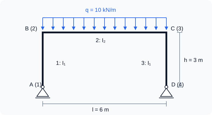
Selected data: l = 6 m, h = 3 m, q = 10 kN/m, E = 200 GPa, A₁ = A₂ = 0.02 m², J₁ = 8·10⁻⁵ m⁴, J₂ = 1.6·10⁻⁴ m⁴. The program denotes second moments of area by I. Density 7800 kg/m³ is required input but does not affect statics; self-weight is not added automatically. Global X points right and Y up. Only member 2 is loaded: 20,2,2,0,-10000.
Drawing reference and axial deformation
With positive downward load intensity q and sagging-positive beam moments:
k = (J₂/J₁)(h/l) = 1; VA = VD = ql/2
H₀ = ql² / [4h(2k + 3)]; HA = +H₀, HD = −H₀
MB = MC = −H₀h; M(l/2) = ql²/8 − H₀h
The drawing formulas neglect axial deformation. Element 113 includes finite EA. An independent force-method solution, releasing the horizontal restraint at D, gives:
H [2h³/(3EJ₁) + h²l/(EJ₂) + l/(EA₂)] = ql³h/(12EJ₂)
H = ql² / {4h[2k + 3 + 3J₂/(A₂h²)]}
Substituting this H in the moment expressions gives the exact reference for the finite-EA model. Equal column shortening does not affect horizontal thrust but is included in the vertical displacements at B and C. The horizontal reaction differs from the drawing by approximately 0.0533%.
| Quantity | Drawing (EA → ∞) | Finite EA, FEM reference |
|---|---|---|
| VA = VD, kN | 30 | 30 |
| HA = −HD, kN | 6 | 5.996802 |
| MB = MC, kN·m | −18 | −17.990405 |
| M(l/2), kN·m | +27 | +27.009595 |
| MA = MD, kN·m | 0 | 0 |
Running the example and checking results
Load CasePinnedPortalUniform.txt with Open TXT in the preprocessor and select Run analysis. Automated verification is in example_08_pinned_portal_uniform.m:
addpath(pwd);
setup;
addpath(fullfile(pwd, 'reference', 'examples'));
r = example_08_pinned_portal_uniform();
exportPostprocessorData(r.model, r.analysis, 'output/pinned-portal-uniform.json');
The example checks all reactions, 18 member end forces, 12 nodal displacements, axial forces, beam section moments, equilibrium, and convergence toward the drawing formula when the beam area increases by a factor of 100. Force tolerance is 10⁻⁷ + 10⁻⁹|reference| in N or N·m; displacement tolerance is 10⁻¹² + 10⁻⁹|reference| in m or rad. It runs as part of test_reference_examples.
Moments in localEndForces act on the element, so for BC: M_B = -f(3) and M_C = f(6). Include the load when recovering the beam diagram: M(x) = −Hh + qx(l−x)/2. Linear interpolation between end moments would miss the positive maximum. Three elements suffice for these forces and nodal displacements; deflection inside the loaded beam additionally requires the particular solution for q or mesh refinement.
Open the supplied JSON result in the postprocessor with Open JSON, then select Overlay → M for the moment diagram.
The original formulas come from the user-supplied fragment titled “Rectangular frame with equal-section columns and pinned bases”. No bibliographic details appear in the fragment. Dimensions and section properties were selected for this example.
Laboratory 03. Axial member extension: displacement and support reaction
The aim is to obtain displacement from equilibrium and explain how one unknown becomes a full vector of four displacements.
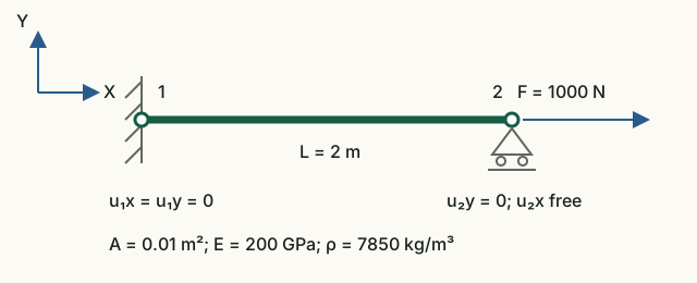
Input data and notation
Length L = 2 m, cross-sectional area A = 0.01 m², modulus E = 200 GPa, force F = 1000 N. Positive X points right. Full-vector order: [u₁x; u₁y; u₂x; u₂y].
| Global DOF | Displacement | Condition |
|---|---|---|
| 1 | u₁x | 0, constrained |
| 2 | u₁y | 0, constrained |
| 3 | u₂x | Unknown, F applied |
| 4 | u₂y | 0, constrained |
Before running: hand calculations
- Identify the free displacement in the diagram and write its global number.
- Calculate the stiffness k = EA/L in N/m. Write the equation k·u₂x = F and find u₂x = FL/(EA).
- Use equilibrium of the entire member to find reaction R₁x. Construct the full displacement vector, inserting zeros at constrained DOFs.
Run in Octave
Run from the project root. The supplied function prints the results; you do not need to edit its code for this exercise.
addpath(pwd);
setup;
addpath(fullfile(pwd, "reference", "examples"));
r = example_03_static_bar();
Working with the results
- In the lines
Fixed DOFsandFree DOFsfind the numbers from your table. Number 3 denotes horizontal displacement of node 2. - Compare
Reduced stiffness Kff [N/m]with your EA/L, andReduced load Ff [N]with force F. Divide the second number by the first: the result should equal the third component ofComplete displacement vector [m]. - Compare the full vector with your prediction and the first component of
Reaction vector [N]with reaction −F. Check R₁x + F = 0. - Use the formula to predict the displacement change when separately doubling L, A and E. Explain why the reaction stays the same at a fixed force.
Kff = 10⁹ N/m, Ff = 1000 N, u₂x = 10⁻⁶ m = 0.001 mm. Full vectors: u = [0; 0; 10⁻⁶; 0] m and R = [−1000; 0; 0; 0] N. Stiffness, force and displacement are related by an equation, so their numerical values cannot be compared directly with one another.
What to include in the report
The diagram with DOF numbering, the hand-derived equation, a quantity/hand calculation/Octave/units table for stiffness, displacement and reaction; explain zero components and predict the three parameter changes.
Chapter source code
solveStatic.m— complete static solution sequence;partitionDOFs.m— free and constrained indices;validateReducedSystem.m— mechanism detection;calculateStaticEquilibrium.m— force and moment balance;createPostprocessorData.m— preparing a validated data structure;exportPostprocessorData.m— safe postprocessor JSON output;postprocessor/index.html— offline visualization and image export;example_03_static_bar.m— executable laboratory.
Checking distributed loads
Consistent element loads enter the full F before solving and calculating R=Ku−F. For a uniform load, the resultant is qL and acts at the midpoint of the original element; global equilibrium is also checked using these original resultants. For a cantilever, |v(L)|=|q|L⁴/(8EI), |θ(L)|=|q|L³/(6EI); free-end forces are zero.
MPC
MPC analysis solves Kr q = Fr and reconstructs full u = Tq. Forces are recovered from the original system, including loads on dependent and fixed DOFs. Global static equilibrium includes both support reactions and MPC forces.
Complete MPC guide · JSON v3 · CaseMPCFrame.txt · CaseMPCTruss.txt