From nodal displacements to forces

Three recovery steps

For element e the function recoverElementResults performs:

u_e = u(dofs_e)

u_local = T_e u_e

q_local = k_local u_local

The first expression selects components using element.dofs, rather than node numbers. The second transforms global displacements into element axes. The third gives generalized nodal forces acting on the element and work-conjugate to its local DOFs.

elementDisplacements = u(element.dofs);
localDisplacements = element.transformation * elementDisplacements;
localEndForces = element.localStiffness * localDisplacements - feLocal;

What static analysis returns

solveStatic places the array elementResults in the result structure. Each element record contains:

Type 112 member

The local displacement order is [u₁; v₁; u₂; v₂]. Axial strain, stress and force are calculated as:

ε = (u₂ − u₁)/L,   σ = Eε,   N = Aσ

Positive ε, σ and N mean tension; negative values mean compression. In tension, local end forces have opposite signs:

q_local = [−N; 0; N; 0]

There is no contradiction: the scalar N describes the member state, while components of q give the force directions at its two ends.

Type 113 frame

Frame local vectors use a consistent order:

u_local = [u₁; v₁; θ₁; u₂; v₂; θ₂]

q_local = [N₁; V₁; M₁; N₂; V₂; M₂]

Each force or moment is positive along its work-conjugate local DOF direction. For example, for a horizontal cantilever of length L and force P in the positive direction of the local axis y at the free end:

q_local = [0; −P; −PL; 0; P; 0]

Element forces and reactions are different quantities

Reactions are calculated in global coordinates for the entire model:

R = K u − F

End forces belong to one element and use its local axes. At a shared node, contributions from several elements are first rotated back using transposed T and summed:

K u = Σ T_e^T q_local,e

The external load is then subtracted from the internal nodal forces. Thus localEndForces cannot be called reactions without transformation and assembly. They coincide directly only in special cases, such as the fixed end of a single horizontal element with no applied nodal load at that end.

Laboratory 07. From displacements to stresses and end forces

The aim is to independently verify two results using member extension and cantilever equilibrium.

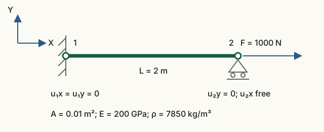
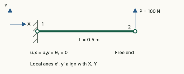
Input data and notation

For the member, use the laboratory 03 data: L = 2 m, A = 0.01 m², E = 200 GPa, F = 1000 N. For the cantilever, L = 0.5 m, A = 10⁻⁴ m², E = 200 GPa, I = 0.33·10⁻⁸ m⁴, P = 100 N upward. Both models are horizontal, with local axes aligned with global axes.

Before running: hand calculations

1. For the member, find σ = F/A, ε = σ/E, ΔL = εL and N = σA.
2. For the cantilever, write Y-force equilibrium and moment equilibrium about node 1. Find R₁y and M₁ with the force direction shown.

Run in Octave

Run from the project root. The supplied function prints the results; you do not need to edit its code for this exercise.

addpath(pwd);
setup;
addpath(fullfile(pwd, "reference", "examples"));
r = example_07_result_recovery();

Working with the results

1. From Truss local displacements [u1; v1; u2; v2] find u₂ − u₁ and divide by the length. Compare strain, stress and axial force with the printed Truss strain, stress and axial force.
2. In Truss local end forces find the two axial components. Explain their opposite signs although axial force N is positive and the member is in tension.
3. Label the six components of Frame local end forces [N1; V1; M1; N2; V2; M2] with units N or N·m. Compare the first three with Frame support reactions, and the last three with the free-end load.
4. Check equilibrium: V₁ + V₂ = 0 and M₁ + M₂ + V₂L = 0. Use linearity to predict the signs of strain, stress, forces and reactions if the load reverses.

What to include in the report

Both diagrams, hand calculations, an analytical/Octave/units table, the two cantilever equilibrium equations, and an explanation of end-force signs.

All laboratories with one command

run_reference_examples runs seven examples in sequence and returns results in fields named after the functions:

addpath(pwd);
setup;
addpath(fullfile(pwd, "reference", "examples"));
results = run_reference_examples();

For a quiet check, use run_reference_examples(false). The runner finds the repository root from its own file, so once the examples directory is on the path it does not depend on the current working directory. Exceptions are not caught: the first failed check immediately stops execution.

Diagrams for loaded elements

For total local intensities qx, qy and end vector f: N(x)=−f₁−qx·x, V(x)=−f₂−qy·x, M(x)=−f₃+f₂·x+qy·x²/2. The postprocessor includes the interior extremum of M. Scalars axialStrain, axialStress, axialForce and the stress returned by StressCalc are average axial quantities, not bending stresses. Displacement geometry retains finite element interpolation.

Results with element loads are exported as JSON v2; legacy v1 results remain supported.

MPC

Each C row has dependent coefficient +1 and master coefficients −c. The residual splits as r = supportReactions + Cᵀλ; mpcForces = Cᵀλ and mpcMultipliers = λ. At a fixed master, the support reaction is r minus the MPC force. For a mode, r = Kφ − ω²Mφ; forces use the stored eigenvector amplitude. The reactions field retains the full residual. JSON v3 labels these quantities separately.

Complete MPC guide · JSON v3 · CaseMPCFrame.txt · CaseMPCTruss.txt

Mz end releases

Complete guide: chapter 4b

Static localEndForces = Klocal*ulocal − flocal uses actual end rotations; released moments vanish within tolerance without overwriting results. JSON v4 carries DOF ownership and element maps. Cards show both rotations; history charts offer element/end/thetaZ. An absent nodal rotation is not shown as zero.

JSON v4 · CaseReleaseStatic · CaseReleaseModal · CaseReleaseTransient

Stresses from section geometry

Assigned sections enable static σmin and σmax diagrams. Select a member, then choose x/L with the slider or numeric input to inspect the oriented section, stress distribution and color scale. Red is tension (+), blue compression (−). The scale stays fixed over the selected member. Its details list numerical extrema and their locations; Export section SVG saves the cross-section image.

Frames use σ(x,η)=N(x)/A−M(x)η/I; trusses use σ=N/A. The in-plane transverse coordinate η is measured from the centroid. Uniform and linear distributed loads are included; interior extrema are found independently of rendering resolution. Legacy mean axialStress retains its previous meaning and does not replace bending stress.

x points from node 1 to node 2. At 0°, y is the in-plane left normal and z points towards the viewer (⊙). The axes are right-handed, drawn near one third of the member length and toggled with Section axes. The tee flange starts at +y, the channel opens towards +z. Rotating 90° changes the active bending axis; 180° flips the profile.

The model remains planar without torsion or eccentricity. Sections also affect mass and stiffness in modal and transient analysis, but new stress results are static only. Members without section geometry have no bending-stress result. Legacy cases and JSON v1–v5 retain their behavior.

JSON v6 and sign conventions · Beam: σmax=750000, σmin=−750000 at x/L=0.5