Average acceleration method

Equation of motion and reduction

The free DOFs satisfy:

M_ff a(t) + K_ff u(t) = F_f(t)

This is the linear undamped special case of a more general equation with damping matrix C and a nonlinear restoring force. In MKE-F, C = 0, there is no nonlinear term, and constrained components of the full histories remain exactly zero.

A single time grid

For step Δt and requested duration T the step count is fix(T/dt). Every returned history has N + 1 columns:

t₀ = 0,   t₁ = Δt,   …,   t_N = NΔt

If T/Δt is not an integer, the actual duration result.duration is shorter than the requested result.requestedDuration. Octave column numbers are one greater than step numbers: column 1 corresponds to t = 0.

Initial state

The user may specify full vectors u₀ and v₀. Their constrained components must be zero. Initial acceleration is not an independent input; it is computed from equilibrium:

a₀ = M_ff⁻¹[F_f(0) − K_ffu₀]

Thus all three initial histories begin from one physically consistent state.

Newmark approximations

Displacement and velocity at the next step are related to accelerations:

u_n+1 = u_n + Δt v_n + Δt²[(1/2 − β)a_n + βa_n+1]

v_n+1 = v_n + Δt[(1 − γ)a_n + γa_n+1]

The choice β = 1/4, γ = 1/2 gives the average acceleration method. For a linear system it is second-order accurate and unconditionally stable, but stability does not guarantee adequate accuracy when Δt is too large.

Effective stiffness

The code uses these coefficients:

a0 = 1/(beta*dt^2);
a2 = 1/(beta*dt);
a3 = 1/(2*beta) - 1;

One system is solved at each step:

K_eff u_n+1 = F_n+1 + M(a₀u_n + a₂v_n + a₃a_n)

K_eff = K_ff + a₀M_ff

The matrix K_eff is constant, so solveTransient performs Cholesky factorization once and reuses it at every step. Acceleration and velocity are updated after solving.

Impulse on the discrete grid

A type 12 load is nonzero only in column t = Δt. For a single-step rectangular pulse:

I_discrete = F₀Δt

When comparing grids with different Δt, preserve the impulse rather than the amplitude: F₀ = I/Δt. Otherwise refining the step changes both the physical excitation and the numerical error.

Convergence and energy

For a free undamped oscillator with ω = √(k/m):

u(t) = u₀cos(ωt) + [v₀/ω]sin(ωt)

Halving Δt should reduce the error of a second-order method by about a factor of four. This is more reliable than a single check at one step size.

Total mechanical energy of the free system:

E(t) = 1/2 v^TMv + 1/2 u^TKu

For a linear undamped problem, the average acceleration method introduces no algorithmic damping, and energy is conserved to rounding accuracy. Under external loading, energy changes through external work, so constant energy is no longer an expected invariant.

Single-sided spectrum

computeSingleSidedSpectrum applies an FFT to each displacement row and returns nonnegative frequencies. For N_s samples:

Δf = 1/(N_sΔt)

The free-oscillator spectral peak should lie near its natural frequency, but finite duration and a frequency falling between discrete bins cause leakage. A reasonable check therefore allows for resolution Δf instead of demanding bitwise frequency agreement.

Running the analysis and viewing results

In Octave, from the project root, run:

addpath(pwd);
setup;

problem = StructFEProblem(fullfile( ...
    'examples', 'cases', 'CaseBeam.txt'));
model = problem.GetAnalysisModel();
result = problem.RunTransient(1e-4, 1e-2, 3, 2);

options = struct(...
    'title', 'Transient response', ...
    'lengthUnit', 'm', 'forceUnit', 'N', ...
    'momentUnit', 'N*m', 'timeUnit', 's', ...
    'transientFields', {{'displacements', 'velocities', ...
                         'accelerations', 'loadHistory', ...
                         'reactions', 'spectrum'}}, ...
    'timeStride', 1, 'prettyPrint', true);
exportPostprocessorData(model, result, ...
    fullfile('output', 'transient-history.json'), options);

Then open postprocessor/index.html by double-clicking in Chrome and drag onto the page output/transient-history.json or select it using Open JSON. A supplied example is in examples/results/transient-history.json. No local server is needed.

Laboratory 06. Free vibration: Newmark accuracy

The aim is to compare numerical and analytical motion and determine convergence order from three grids.

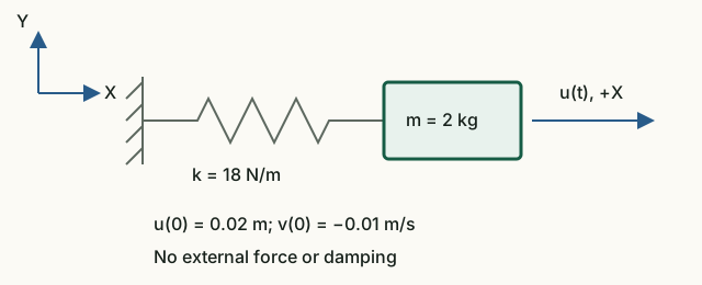
Input data and notation

m = 2 kg, k = 18 N/m, u₀ = 0.02 m, v₀ = −0.01 m/s. Force and damping are zero. The supplied example calculates three periods with 50, 100 and 200 steps per period; β = 1/4, γ = 1/2.

Before running: hand calculations

1. Find ω = √(k/m), f = ω/(2π), T = 1/f and the initial acceleration a₀ = −ku₀/m.
2. Write u(t) = u₀cos(ωt) + (v₀/ω)sin(ωt). Find the initial energy E₀ = mv₀²/2 + ku₀²/2.

Run in Octave

Run from the project root. The supplied function prints the results; you do not need to edit its code for this exercise.

addpath(pwd);
setup;
addpath(fullfile(pwd, "reference", "examples"));
r = example_06_newmark_sdof();

Working with the results

1. Compare Natural frequency, period and Initial acceleration with your calculation.
2. From Steps per period and maximum displacement error record the three errors. Calculate the 50-step/100-step and 100-step/200-step error ratios. Why does a ratio near four indicate second order?
3. Use the commands below to plot exact and numerical motion on the finest grid, then their difference. A separate difference plot reveals errors even when the original curves appear identical.
4. Compare Relative energy drift with the motion error. Explain why energy conservation does not imply exact phase agreement.
5. Compare Spectrum peak with the natural frequency: the difference should be within the printed bin width. Using the formula Δf = 1/(NΔt) predict the effect of shortening the recording duration at the same step size.

After running, execute in Octave with a graphics window available:

figure;
plot(r.time, r.displacements(1,:), "-", ...
     r.time, r.exactDisplacement, "--");
xlabel("t [s]"); ylabel("u [m]");
legend("Newmark", "Exact"); grid on;
figure;
plot(r.time, r.displacements(1,:) - r.exactDisplacement);
xlabel("t [s]"); ylabel("u - u_exact [m]"); grid on;

For a headless run, record a few value pairs and their differences instead of plotting:

idx = round(linspace(1, numel(r.time), 13));
disp([r.time(idx).', r.displacements(1,idx).', ...
      r.exactDisplacement(idx).', ...
      (r.displacements(1,idx) - r.exactDisplacement(idx)).']);

What to include in the report

Hand calculations, the errors and their ratios, two plots (or a value table for a headless run), an explanation of energy conservation versus motion accuracy, and a conclusion about spectral resolution.

MPC

Newmark integrates independent coordinates with Kr, Mr and TᵀF(t). Displacement, velocity and acceleration are reconstructed with T. Initial displacement and velocity must satisfy SPC and MPC constraints; incompatible values are rejected. Dynamic constraint forces use r = Ma + Ku − F.

Complete MPC guide · JSON v3 · CaseMPCFrame.txt · CaseMPCTruss.txt