Natural frequencies and mode shapes

Generalized eigenvalue problem

For free motion without external force:

M ü(t) + K u(t) = 0

Substituting the harmonic form u(t) = φ sin(ωt) gives:

K φ = λ M φ,   λ = ω²

The natural angular frequency is ω = √λ, and the frequency in hertz is:

f = ω/(2π)

In solveModal pairs are computed using eig(Kff, Mff), then sorted in ascending λ order.

Why solve only on free DOFs?

As in statics, first construct fixedDOFs and freeDOFs. The eigenvalue problem uses the reduced matrices:

K_ff φ_f = λ M_ff φ_f

Keeping constrained components in the full problem by artificially modifying rows makes the spectrum depend on the numerical constraint method. Reduction preserves the physical matrices of the free subsystem.

validateReducedSystem checks positive definiteness of K_ff and M_ff. A mechanism or massless free DOF stops the analysis before calling eig.

Returning to the full mode shape

Each reduced eigenvector is expanded to all model DOFs:

modeShapes = zeros(numberOfDOFs, numberOfModes);
modeShapes(freeDOFs, :) = reducedModeShapes;

Constrained DOF rows are therefore exactly zero, and row numbers again match global DOF numbers. This matters for subsequent visualization and comparison of nodal mode shapes.

Mode shape scale and sign

If φ is an eigenvector, then cφ for any nonzero c describes the same mode. The absolute amplitude and sign returned by eig are not physical displacements.

Two useful normalizations:

• mass normalization: choose the scale so that φ^TMφ = 1;
• for display: divide components by max|φ_i| and, if needed, fix the sign of the largest component.

Distinct modes of a symmetric system are orthogonal with respect to mass and stiffness:

φ_i^TMφ_j = 0,   φ_i^TKφ_j = 0,   i ≠ j

Animating a mode in the postprocessor

Save the model and modal result to JSON and open it in the MKE-F offline postprocessor without a local server or internet connection.

1. Run and export

Open a terminal in the project root, start GNU Octave, and run:

addpath(pwd);
setup;

problem = StructFEProblem(fullfile( ...
    'examples', 'cases', 'CaseBeam.txt'));
model = problem.GetAnalysisModel();
result = problem.RunModal();

exportPostprocessorData(model, result, ...
    fullfile('output', 'modal-frame.json'), ...
    struct('title', 'Mode shapes', ...
           'lengthUnit', 'm', 'prettyPrint', true));

After execution, the file modal-frame.json appears in the directory output. You can also check computed frequencies in the terminal with result.frequenciesHz.

2. Open the result

1. Open postprocessor/index.html in Chrome, Edge or Firefox.
2. Click Open JSON and select the generated file output/modal-frame.json. You can also drag it into the dashed area. A supplied example is in examples/results/modal-frame.json.
3. In the Mode list, select a mode. Its frequency f in Hz and angular frequency ω in rad/s are displayed alongside.
4. Click Play to start the animation. The buttons −1 and +1 move to adjacent modes; Visualization speed changes playback speed.
5. Move Phase factor from −1 to +1 to inspect the negative peak, undeformed geometry and positive peak manually. The field Display multiplier changes only the displayed mode scale.
6. Click a node or element: the Selection panel shows normalized components of the selected mode and their values at the current phase.
7. Click Export SVG or Export PNG to save the current frame with the mode number, frequency, phase and scale.

The viewer standardizes the arbitrary sign of each mode and normalizes it for display only. The display factor changes the visible amplitude but not the computed natural frequencies.

SVG or PNG export captures the current visible phase. The caption records the mode number, f, ω, phase factor and scales so the saved frame remains unambiguous outside the application.

Mode residual

A frequency alone does not verify its vector. For each eigenpair, calculate:

r_i = K_ffφ_i − λ_iM_ffφ_i

A relative norm scaled by the sizes of the two terms is useful because it is independent of arbitrary mode scaling. Do not apply this check to full constrained rows: these contain constraint forces analogous to static reactions.

Laboratory 05. Frequencies and modes of a beam with an intermediate support

The aim is to connect free DOFs to mode-shape components and verify frequencies through modal stiffness and mass.

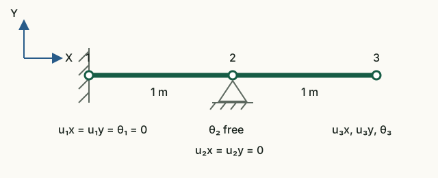
Input data and notation

Each span is 1 m long. A = 4·10⁻⁴ m², E = 200 GPa, ρ = 7800 kg/m³, I = 5.33·10⁻⁸ m⁴. Full component order: [u₁x; u₁y; θ₁; u₂x; u₂y; θ₂; u₃x; u₃y; θ₃]. Modal analysis does not use the external force in the input file.

Before running: hand calculations

1. List constrained and free DOFs from the supports in the diagram. Determine how many frequencies will be found.
2. From Kφ = ω²Mφ derive how frequencies change if all mass doubles at unchanged stiffness.

Run in Octave

Run from the project root. The supplied function prints the results; you do not need to edit its code for this exercise.

addpath(pwd);
setup;
addpath(fullfile(pwd, "reference", "examples"));
r = example_05_modal_frame();

Working with the results

1. Compare Fixed DOFs and Free DOFs with your numbering. In Full modes scaled to max(abs(component)) = 1 each column is a separate mode; label the four unconstrained rows by physical component.
2. For each frequency in Natural frequencies [Hz] calculate (2πf)². Compare with the corresponding diagonal entry of Phi' * Kff * Phi after mass normalization.
3. Check that Phi' * Mff * Phi after mass normalization is close to the identity matrix. Explain the unit diagonal and small off-diagonal entries.
4. Use rows 6–9 of the printed modes to identify the axial mode and the bending modes. Sketch free-end displacement and rotations for one bending mode. The scale and overall sign are arbitrary; the values do not give forced-motion amplitudes.

What to include in the report

The diagram and DOF list, a mode number/f/(2πf)²/modal stiffness/motion type table, a sketch of one mode, and the predicted mass effect.

MPC

MPC analysis solves Kr φr = ω²Mr φr, then φ = Tφr. The mode count equals the number of independent DOFs. Intermediate transverse constraints remove spurious mechanisms in a refined truss member. Nonzero rhs is rejected.

Complete MPC guide · JSON v3 · CaseMPCFrame.txt · CaseMPCTruss.txt

Mz end releases

Complete guide: chapter 4b

Private rotations retain the original consistent mass. The release condition is checked using K*phi − omega²*M*phi in modal analysis and M*a + K*u − F in transient analysis. The elastic K*u moment alone need not vanish. Shapes use end rotations, including modes with stationary nodes.

JSON v4 · CaseReleaseStatic · CaseReleaseModal · CaseReleaseTransient